Plotting

Plotting Example

You can use matplotlib to visualize kinematic relationships.

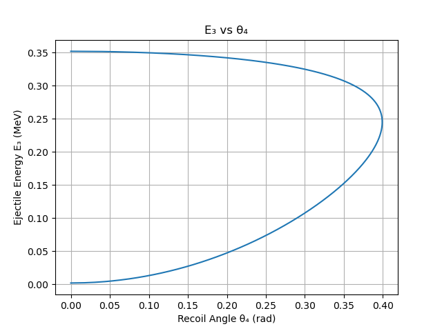
Example: Ejectile Energy vs Recoil Angle

from reaction_kinematics import Reaction
import matplotlib.pyplot as plt

# or equivalently: Reaction("3H(p,n)3He")
rxn = Reaction("p", "3H", "n", "3He")

data = rxn.kinematics_table_at_beam_energy(1.2)

plt.plot(data["theta4_lab"], data["energy3_lab"])
plt.xlabel(f"Recoil Angle θ₄ ({data.units['theta4_lab']:~})")
plt.ylabel(f"Ejectile Energy E₃ ({data.units['energy3_lab']:~})")
plt.title("E₃ vs θ₄")
plt.grid(True)
plt.show()

It should return a graph like this:

The axis labels are built from data.units[...] (~ gives the short form, e.g. "MeV" instead of "megaelectron_volt"), so they stay correct if you change angle_unit/energy_unit.

---

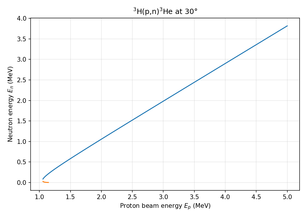
Kinematic Curves at Fixed Lab Angle

kinematics_curve_at_angle sweeps over a range of beam energies at a fixed ejectile lab angle (theta3_lab), returning ejectile kinematics for both solution branches.

import numpy as np
import matplotlib.pyplot as plt
from reaction_kinematics import Reaction

# or equivalently: Reaction("3H(p,n)3He")
rxn = Reaction("p", "3H", "n", "3He")
beam_energy_array = np.linspace(1.0, 5.0, 500)
theta3_lab = 30  # fixed ejectile lab angle (degrees)
branches = rxn.kinematics_curve_at_angle(beam_energy_array, theta3_lab)

for branch in branches:
    plt.plot(branch["beam_energy_lab"], branch["energy3_lab"])

plt.xlabel(f"Proton beam energy $E_p$ ({branches[0].units['beam_energy_lab']:~})")
plt.ylabel(f"Neutron energy $E_n$ ({branches[0].units['energy3_lab']:~})")
plt.show()

Each call returns a list of two KinematicsResults (branch 0 = high-energy solution, branch 1 = low-energy solution), each with arrays for beam_energy_lab, energy3_lab, energy4_lab, theta4_lab, velocity3_lab, velocity4_lab, momentum3_lab, momentum4_lab, jacobian3_lab, and jacobian4_lab. Where a branch does not exist the values are NaN.

The full example script is at examples/kinematic_curve_example.py.

---